Playing with Matches -Revisited
Warning Mathematics Ahead
Paul McMahon VK3DIP
Abstract:
A brief survey of the various matching techniques available to match the transmission line to the Antenna with particular reference to those methods suited to use with Yagi style antennas. This part concentrates on the theory of the various matching techniques.
Introduction to revised version.
About 10 or 11 years ago I started to write what was intended to be a series of articles for an amateur radio magazine on antenna matching. Due however to some comments from various people that they were way too technical the idea got shelved. I had however by then written the first one and a bit, so when putting together the YagiCAD website I added PDF copies and the associated excel spreadsheets in a miscellaneous section to pad the site out. Fast forward to now, while YagiCAD has attracted by far the most email traffic, I have also had quite a few positive comments on the matching papers, so when I finally got around to taking a position on the great Gamma match debate ( I ended up giving up on Dr Balanis and siding with the ARRL), and thus needed to redo the match routines in YagiCAD, I also decided to revise this what was the first article.
Introduction.
Some time back I was looking for some information on antenna matching to add in to my Yagi design and analysis program YagiCAD (Ref 1), and I found that apart from references such as the ARRL Antenna handbook (Ref 2) there appeared to be little written recently about the various matching techniques used by Amateurs. In particular the ARRL texts were for the main part based on articles written in the late 60’s and early 70’s (Refs 3&4) and were heavily biased towards the use of graphical methods such as Smith Charts and published curves. Whilst these techniques are just as valid today as then, they didn’t really give me a good feeling for what it was that I was trying to do when matching an antenna. Having gone to the trouble of researching this topic and doing the several pages of mathematics involved I thought that perhaps other Amateurs might be interested in some of the results. These results are of course basically the same as those found in other references but by use of the computing power available to the average Ham on his personal computer today, perhaps more insight is available.
Basic Antenna Model
The basic antenna, or antenna element, can be modelled as a resistive component in series with a reactive one. The values, and sign in the reactance case, vary with frequency, element diameter, length, and spacing to other elements or ground, but for a particular antenna at one frequency they can be considered constant. How you determine these values is another matter, about which we shall discuss more latter, but for the moment we will consider the simple fixed case. An example is shown in Figure 1 Physical, and Figure 2 Equivalent Circuit.
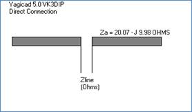
Figure 1 - Physical Driven Element
Figure 2 - Circuit Model
Here we see a dipole element (in this case a part of a three element Yagi array from Yagicad) which has an input impedance of 20.07 Ohms resistance (Ra) in series with a negative or Capacitive reactance of 9.98 Ohms (Xa) . Mathematically we would write this as the complex impedance:
![]()
Where
![]()
In a real world case of course the value of Ra would be made up of the radiation resistance (where the power is dissipated into radiating waves in the transmitting case) and a (hopefully small) value of material loss due to non-ideal conductors. For the purpose of the simplistic analysis here we will assume this loss component is zero.
It is worth noting here the effect that varying the element length will have in the most common case where the antenna element is about one half wavelength long. At exactly one electrical half wave long the element is said to be resonant and has Xa equal to zero. Slightly shorter than this is said to be below resonance and will produce a negative or capacitive reactance value for Xa, slightly longer is above resonance and will produce a positive or inductive reactance. The value of Ra tends to be less dependent on length and more dependent on spacing to other elements and the like.
What is a Match?
For my purposes here I am defining a match as something which will have a VSWR as close as possible to 1 to 1 at the antenna transmission line interface. With a transmission line impedance of Ro Ohms the VSWR for our model element is as given by :
![]()
Where
The simplest sort of match would be one where we have arranged for G to be 0 ie. the VSWR is one. We could do this by having the intrinsic impedance of the transmission line equal to the resistive component of the antenna impedance and with an antenna reactance of zero, ie. resonance. While it is reasonably easy to achieve resonance by just shortening or lengthening the antenna element, the value of Ra is not so simply varied, even using genetic techniques. This is especially true as the number of elements on a Yagi is increased, especially if you are trying to optimise other factors such as gain at the same time. Values for Ra of below 30 Ohms, ie. well under the 50 Ohms of commonly available transmission lines, are the norm. We could of course just add some resistance in series to make this up but apart from exceptional cases were broad-banding is more important than efficiency (power absorbed by this additional resistor is dissipated as heat) this is usually not done. There is of course also the question of balanced versus unbalanced transmission line and load but we will leave that complication for a bit later and for the moment assume everything is balanced.
The Discrete L ( a.k.a. Beta), Discrete C, and Hairpin Match.
The simplest matching method that would normally be called such, and that is commonly used, is to place a reactance in parallel with the antenna. The addition of this reactance apart from any resistive or dielectric losses in the inductor or capacitor will not lower the efficiency of the antenna, but will to some extent step up the effective value of Ra as seen by the transmission line. The physical and circuit model for this case would be as shown in Figure 3 and Figure 4.
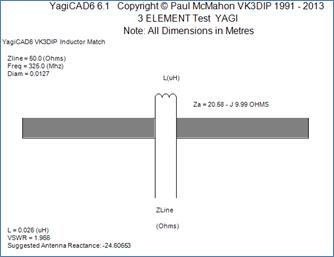
Figure 3 – L Match for Za = 20.58 –J9.99
Figure 4 - Circuit Model
It should be noted that, because using a shunt inductor is the most common, the figures here show the shunt as inductive and the antenna reactance as capacitive. The analysis here however will be kept general and is equally valid for the case of an inductive antenna and capacitive parallel reactance.
It makes the mathematics easier if we consider the input admittance rather than impedance, which in this case can be shown to be:
![]()
A little bit of rearranging and separating into real and imaginary parts gives:

In the case we are aiming for, the reactance will be zero, which is true for either impedance or admittance, and the input impedance should equal the impedance of the transmission line, so assuming we arrange things to be at this optimum matching point then we can come up with some interesting results:

Equation 1
![]()
Equation 2
Equation 3
These equations let us draw a number of conclusions:
1. Equation 1 tells us this is a step up only situation with the amount of step up being proportional to the magnitude of antenna reactance squared, if the element is resonant, ie Xa = 0, there is no step up, and no match.
2. Equation 1 and Equation 2 tells us this match won’t work if Ra is greater than Ro.
3. Equation 2 gives us the optimum value for Xa, it tells us that for given values of Ra and Ro there are only two possible values of Xa which will allow a perfect match. If Xa is not right then this match cannot be perfect, irrespective of Xm.
4. Equation 3 tells us what Xm we will need to complete the match and also that a negative Xa will require a positive (Inductive) Xm and a positive Xa will require a negative (Capacitive) Xm.
In our example (Figure 3) using these equations the reactance value of the antenna element is not high enough at the moment to allow a match to 50 Ohm transmission line. Ie. from Equation 1 with the values shown the best obtainable Ro would be:
![]()
The best Ro of just over 25 Ohms leads to the VSWR as indicated by YagiCAD as just under 2:1.
Again forget about the unbalance for the moment. We could shorten the element to raise this value, but this may also effect the Ra value, and possibly affect the overall antenna performance, ie. gain and pattern. Doing this by cut and try on a real antenna could be quite time consuming and possibly ultimately a waste of time. This is why some sort of computational model of the antenna where you can easily try these things without having to build it really helps out. In this case using Equation 2 above gives an optimum version of Xa. We can then use something like YagiCAD to vary our yagi ( shorten the driven element) to achieve this value. This process is iterative as shortening the driven element as well as increasing the reactance (Xa), also changes the radiation resistance (Ra), in this case decreasing it. This decreased value of Ra then leads to a new optimal value for Xa which again requires varying the length of the driven element and so on. YagiCAD has an option to just keep doing this until the VSWR is reasonable (the auto adjust option). This was done in Figure 5 and you will see that the value of Xa we ended up with was -23.31 Ohms with an Ra of 16.1 Ohms (which is somewhat decreased from our original value of 20 Ohms)
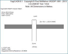
Figure 5 - Optimal L Match Physical
We can see that the VSWR now obtained is at a very reasonable value of 1.003:1.
We can see that slightly decreasing the element length has increased the reactive component, and decreased the resistive component. Luckily it has also had minimal effect on Gain and Front to Back, so we could just stick with this and build it using a coil of 0.017uH. This match is a discrete L match, which is sometimes also called a Beta Match. In some cases, especially at VHF, it may not be physically desirable to wind a discrete coil, in this case we could simulate this inductance using a short section of shorted parallel wire transmission line, called a stub or in this case more usually called a hairpin. For a section of shorted parallel wire transmission line of electrical length less than one quarter wavelength the impedance at the open end will be inductive and given by the formulas below.
![]() where
where
![]()
and

where; l = length of stub, l = Wavelength, S = Centre to centre spacing of the two parallel wires, and d = the wire diameter, all in metres.
Applying these to the example here gives the Hairpin match shown in Figure 6.
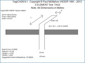
Figure 6 Optimal Hairpin Match Physical
It is worth noting again that while we have shown inductive shunt matching here exactly the same thing would be possible (with a positive value of Xa) with a Capacitive shunt either formed of a discrete capacitor or Open (as opposed to shorted) transmission line, or set of physical plates.
For completeness and because we will need it later we should also continue the mathematical analysis of our model ( Figure 4) to get the more general case of the resultant input impedance, which after considerably more manipulation and separating into real and imaginary components can be shown as:
![]()
Equation 4
Which if again we set Rin to the required input impedance Ro and only consider the real component, we can then arrange this into a standard quadratic form for Xm .
![]()
Equation 5
Which can be solved for Xm using the normal quadratic formula using:
![]()
Where
![]()
![]()
![]()
What to do if you can’t get the right value of Xa.
To illustrate what we are doing here let us consider the general case, of Equation 4. and what happens to the input impedance as the value of Xm varies. This is shown graphically in Figure 7 and Figure 8 derived using an MS Excel spreadsheet (Ref. 5. (Xmatcha.xls))
Figure 7 - Graphs of Rin and Xin versus values of Xm for the initial case Ra = 20.2, Xa= -9.98
Note the blue line which is the calculated input resistance which in Figure 7 you will see never gets to the required Ro value no matter what value of Xm is used. In fact the highest or closest we get in this case is the about 25 Ohms (as per the above calculation and the approx 2:1 VSWR as found by YagiCAD earlier).
In Figure 8. We see the case where we have varied the Xa (and thus Ra) to get what we called an optimal match.
Figure 8 - Graphs of Rin and Xin versus values of Xm for the optimal case Ra = 16.1, Xa= -23.3
Note that in this case the blue line is just touching the required 50 Ohms level just as the pink reactance line crosses zero. This is the Optimal case. This corresponds to a reactance value of the matching component of some 34 Ohms which at the frequency of interest, leads to the 0.017uH lumped L or hairpin as previously shown.
To explore other types of matches let us consider the case of the above antenna if for some reason we wanted to match to, say, 40 Ohms. In this case from Figure 8 we can see that the Rin component crosses 40 Ohms in two places at approximately Xm = 25 and 53 Ohms. The problem here is that in both of these cases there is a non-zero value of input reactance of approximately Xin = +20, and – 20 Ohms respectively. If we wanted to stick with the values of antenna impedance we had here then what we need to do is to pick one or the other of these value pairs and cancel out the unwanted reactance. For practical reasons if we wanted to actually achieve this match we would probably pick the smaller value of Xm leaving a reactance of +20 Ohms to be cancelled out. In this case the simplest way to cancel this out would be by using a pair of series capacitors each of reactance –10 Ohms, one coming from each side of the shunt Inductor going to the transmission line. We need to split the capacitance into two to maintain the assumed balance of our transmission line. The resulting circuit is illustrated in Figure 9.
Figure 9 - Resulting circuit showing cancelling Capacitors.
In this special case, even if we cannot get the right antenna reactance value it is still possible to obtain a match by the addition of further matching components. These additional reactive components, again assuming low dielectric losses etc., will not adversely affect the efficiency of the match at the actual frequency of design. However all of these extra components have frequency dependant reactance, the resultant circuit has a Q, and is actually in this case a high pass LC filter.
The Gamma and Tee Match.
In the preceding section we saw that under some circumstances the addition of simple series components could make a match when it was otherwise not possible. The practical problem is that usually we need much higher step-up ratios to make this work with real transmission lines and there is a limit to how far we can go with just shortening or lengthening the element to make the antenna reactance bigger. The way to get higher step-up ratios is to use some form of transformer action. While discrete broad-band transformers can be made or bought, this approach is rarely used outside of receiving only antennas because of saturation problems even at low power levels. It is also possible to use a transmission line quarter wave transformer but this is limited in its usefulness by the small number of values of transmission line impedance commercially available. You can of course make your own but this can get mechanically difficult. The most common method used to provide a transformer action is to introduce a wire or equivalent additional element parallel with, and in close proximity to, the radiating antenna element so as to form a section of transmission line. If this is done on only one side of the driven element dipole we call it a Gamma match (the Greek letter Gamma is an upside down L), if it is on both sides we call it a Tee Match. Both of these cases have the additional advantage of not requiring the antenna element to be broken in the middle leading to a mechanically stronger antenna. Also if only one side of the element is treated in this way the match removes the need for some form of unbalanced to balanced transformation if an unbalanced form of transmission line such as coax is used.
The single biggest problem with this sort of matching technique is that the only practical way to model it is to reduce it to an equivalent lumped element model similar to those above. This is a problem because clearly the Gamma or Tee arm is actually going to be part of the antenna radiating system and will by its presence have some effect on the antenna properties, which in turn will affect how good a match we have. In practice while the lumped matching model shows good alignment with real world builds for real lumped elements such as coils or capacitors, in the case of the Gamma and Tee the results obtained should only be treated as a rough guide. In fact even the Gamma models given below are subject to debate with fundamental items such as should the antenna impedance be halved or not, with some texts going one way and others the other. For the models below I have sided with the current ARRL antenna handbook, as that approach I have found produces results closest to some special case tests I have done with NEC2. See the appendix for some example comparisons.
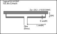
Figure 10 - TEE No C
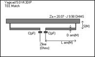
Figure 11 - TEE Match
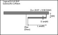
Figure 12 - Gamma No C
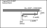
Figure 13 - Gamma Match
These sorts of matches are diagrammed in Figure 10 to Figure 13, which show both the common form of the Gamma and Tee matches, which have the series capacitors, and the less common no C forms.
If we analyse the standard Gamma shown in Figure 13, the equivalent circuit model is as shown in Figure 14 .
Figure 14 - Gamma Match Equivalent Circuit
As can be seen the gamma arm provides both a current transformer action, while also providing a value of effective shunt inductance. This circuit can be simplified somewhat by evaluating the impedance marked as Z2 in Figure 14 to give the version shown in Figure 15.
Figure 15 - Gamma taking into account the transformer action
If we compare this with Figure 4 and the equations which followed we see that we have increased both the effective value of antenna reactance and the antenna resistance, both of which should make it easier to obtain a match to real world transmission lines.
In this form this equivalent circuit can be seen to be identical to the beta or L match case but with the antenna driven element impedance being stepped up by a factor of (1+α)2. As such the previous equations still apply with the addition of this step up factor.
For example Equations 1-3 can still be applied with substitutions of:
Xm ®Xg
Ra ® (1+α)2*Ra
Xa ® (1+α)2*Xa
In the case of Equation 1-3 we have also assumed a zero reactance for input as well, so in this case we are actually looking at a special case of the Gamma match without the need for a series capacitor. This is a perfectly valid possibility, if not often used because of the limited range of antenna impedances it is workable with, in the YagiCAD case this is known as a “Gamma no C” match.
Note as per Equation 2 above with the gamma substitutions for a no C match to be workable the following condition must be met:
![]()
Equation 6
The (1+α)2 step up factor can be found using:
 and
and ![]()
where
 and
and ![]()
![]()
![]()
R = Radius of the Driven Element, r = Radius of the matching Arm, S = Centre to Centre spacing of the Element and Arm, l = Wavelength, l = length of Gamma arm. All in Metres.
The other cases such as the Tee can be similarly analysed and a similar result obtained. See Figure 16. The equations turn out identical except for the Xm = Xg = 2xXt ie. twice the inductive reactance. In effect a Tee match is simply two Gamma matches one on each side, effectively feed in series.
Figure 16 TEE Match Model Circuit
While the step up factor (1+α)2 looks complicated it is worth while looking at a few particular cases to give some guidance. If the arm and element diameters are the same then independent of the spacing the step up factor always works out to be exactly 4. Which is perhaps what we would have expected from the case of the folded dipole which is in itself just a special case of a TEE no C where the arm length = element length/2. We can see this in Figure 17 for three cases of U which is effectively the radius of the antenna element relative to the radius of the match element. Ie. the U=1 case is the one we have already discussed where when the arms are the same the step up = 4 irrespective of the spacing. U = 0.5 means the element radius is half of the match arm radius (the match arm is 2 times the size of the element), U = 1.5 means that the element radius is 1.5 times the radius of the match arm. The spacing is also measured here in units of match arm radius.
Figure 17 - Step Up Factor
So we can see that to get step ups less than 4 the match arm needs to be fatter than the driven element and to get numbers greater than 4 the match arm needs to be thinner than the driven element. Even with this however there is not a great amount of variation in the step up ratio.
If we were then to again look at Equation 6 and taking the usual case of the required Ro of 50 Ohms, and a typical step up of 4, then we can see that the Gamma no C case is restricted to instances where the Ra value is less than 50/4 = 12.5 Ohms. Which is of course possible in some cases where you have gone for high gain, but mostly these days designs target higher values of Ra than that.
The design procedure for the more usual Gamma match with the capacitor is to:
1. Substitute the following in Equations 4 and 5
· Xm ®Xg
· Ra ® (1+α)2*Ra
· Xa ® (1+α)2*Xa
2. Solve for Xg using the quadratic, of Equation 5, and the equation for α above, with values chosen for element diameters and spacings.
3. Using calculated Xg to obtain the length of the arm from the tan and Zo equations above.
4. Substitute back into the imaginary part of Equation 4 to obtain the residual reactance.
5. Cancel this reactance out with the opposite signed series reactance (usually a capacitor).
If we now have a look at this graphically with our original antenna element and taking some arbitrary values for the diameters and spacings we come up with the graph in Figure 18. (using Ref 5. (Gmatcha.xls))
Figure 18 Zin for the Gamma Match case Za = 20.02 - J9.96, Diams = 10mm, S = 30mm
Physically this will look like Figure 19.
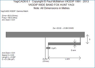
Figure 19 - YagiCAD calculated Gamma Match
In Figure 18 we see that a match to 50 ohms is available ( Blue line crosses Orange line) at an arm length of approximately 0.05 wavelengths but at this point we have a residual reactance of about 50 Ohms ( Pink line) which must be cancelled out with some series C of –50 Ohms. There is also a match point out at greater than 0.2 wavelengths but this would require series inductance to cancel out the residual negative reactance, and in this case this second length would probably be greater than that of the driven element arm (typically around 0.25 Wavelengths).
A close look at this curve shows why can sometimes be difficult to adjust a gamma match. Even small changes in the arm length can lead to big changes in the reactance. This means you would then have to correspondingly adjust the series capacitance before a reasonable VSWR would be obtained. The two adjustments would be interactive and you would end up having to do a series of iterations, with the chances of missing a VSWR dip being reasonably high. A worse case would be if you were trying to match to over 100 Ohms, where it can be seen that no matter what you did with the C or arm length with this set of values you could never obtain a good match.
The above curve is based on a negative value of antenna reactance, the Gamma match will also work if the reactance is positive. Figure 20 gives a graph of this case.
Figure 20 - Gamma match curve with +ve Reactance
|
Driven Element |
Matching Arm |
Required Trans. Line |
||||||||
|
Ra(Ohms) |
15 |
Diam(M) |
0.0127 |
Ro (Ohms) |
50 |
|||||
|
Xa(Ohms) |
3 |
Space(M) |
0.03 |
|||||||
|
Diam(M) |
0.0127 |
|||||||||
From this graph we see that there is indeed a match point out at 0.135 wavelengths with a residual reactance of some 26 Ohms. What we can also see from the graph is that this Gamma arm length is much longer than in the negative antenna reactance case but that the residual reactance is much more well behaved and would probably require much less iteration to get a good match. An examination of a number of other cases shows this as a general trend ie. Negative values of Xa produce the shortest arm lengths and have the option of an ideal value (which will require no series C) but conversely if there is uncertainty on the impedance, the adjustments will be more fiddly. As the antenna reactance moves down to zero (ie resonance) and through to positive values the arm length gets longer and the cancelling C becomes better behaved.
The Omega Match
Another variation on this theme is the Omega Match which has some shunt C as well as the series C . If you do the math you see that the main effect of the shunt C is to enable the same match to be made with less effective inductance and thus shorter lengths of Gamma Arm. Most of the time this is not an advantage unless you are stuck with a positive value of antenna reactance which requires arm lengths greater than the half-length of the element itself. It can however occasionally save a bit of rework if you have a Gamma match that just won’t come in. If you then just temporarily tack the additional capacitor on, and the match then works, this is a sign that the reactance may be a bit more positive than you had designed it to be and you can either leave the C there or shorten the element a bit. Using our example element again a nominal Omega match could be as shown in Figure 21.
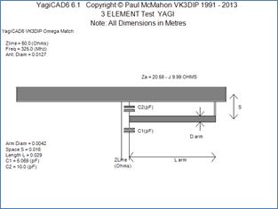
Figure 21 - Omega Match example
With the matching graph from reference 5 (OMatcha.xls) shown in Figure 22.
Figure 22 - Omega Match Curves
|
Driven Element |
Matching Arm |
Required Trans. Line |
|
||||||||||
|
Ra(Ohms) |
20.58 |
Diam(M) |
0.00423 |
Ro (Ohms) |
50 |
|
|||||||
|
Xa(Ohms) |
-9.99 |
Space(M) |
0.0158 |
||||||||||
|
Diam(M) |
0.0127 |
C2(pF) |
10 |
||||||||||
Conclusions .
Hopefully this article will have helped to remove a few of the mysteries surrounding the area of matching the line to the antenna. The idea here is not so much that people necessarily need to be able to calculate things from first principles. With some idea however as to what is happening inside the match, people should be less likely to waste hours working on a match design that could never have worked with that antenna.
73
VK3DIP
References
1/ YagiCAD –Yagi design and analysis program by VK3DIP, Freeware as of version 5 available from http://www.yagicad.com
2/. ARRL Antenna Book , American Radio Relay League Inc.
3/. D.J. Healy, III, W3PG “An Examination of the Gamma Match.”, QST April 1969 pp11-15
4/. H. F. Tolles W7ITB, “How to design gamma-matching networks” , Ham Radio May 1973 pp 46-55
5/. MS EXCEL Spreadsheets Xmatcha.xls, Gmatcha.xls, Omatcha.xls, which implement the equations etc. discussed in this article. They are available from http://www.yagicad.com
Appendix. - Some NEC2 comparisons
Step 1. A Straight dipole.
A simple straight dipole is modelled using a NEC2 based engine (4NEC2) in free space to get the nominal input impedance which will be the Ra + jXa value for these tests.
For convenience I have chosen to do this at a frequency of 299.8MHz as this works out that the wavelength is exactly 1 metre. ie. the dimensions in metres are then also the dimensions in wavelengths. This is done with a length that is close to resonant and a radius of 1mm (diameter 2mm, or 0.002 wavelengths). This model is represented in Figure 23.
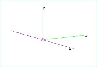
Figure 23 Straight Dipole Model.
When run this model in 4NEC2 with a F= 299.8MHz, L/2 = 0.236m( ie. L = half wave dipole), and radius = 0.001m, we get a value for Za of 70.8 – j 4.06 , which is basically what textbook theory for a classical thin half wave dipole would have predicted.
Step 2. Model of a Gamma Arm on the Dipole, all elements equal radius = 1mm, spacing = 25mm
The next step was to make a NEC2 model of a Gamma Arm on the Dipole from step 1. This basically looks like Figure 24.
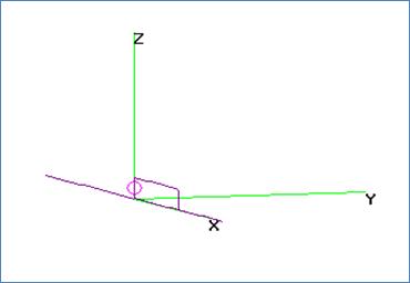
Figure 24 Gamma Arm NEC2 Model
The model parameters were set up as per step 1 ie. F = 299.8MHz, Free space, Dipole L/2 = 0.236m, rad = 0.001m. The Arm spacing is fixed at 25mm and arm diameter is the same as the Dipole. There was a variable defined for the arm length so that the model could be rerun several times with different arm lengths.
The following results were obtained:
|
Arm Wavelengths |
|
|
Zin G (Nec2) |
|
|
0.01 |
1.98+53.9j |
|
0.02 |
8.12+84.5j |
|
0.03 |
19.4+114j |
|
0.04 |
37.6+144j |
|
0.05 |
64.7+173j |
|
0.06 |
103+200j |
|
0.07 |
152+217j |
|
0.08 |
210+219j |
|
0.09 |
267+199j |
|
0.1 |
311+161j |
|
0.11 |
334+115j |
|
0.12 |
338+71.4j |
|
0.13 |
330+37.6j |
|
0.14 |
316+14.8j |
|
0.15 |
300+1.48j |
|
0.16 |
286-4.56j |
|
0.17 |
274-5.43j |
|
0.18 |
264-2.72j |
|
0.19 |
258+2.48j |
|
0.2 |
254+9.44j |
Table 1- Gamma Results from NEC2
Step 3. Model of a Tee Match on the dipole, all elements equal radius = 1mm, spacing = 25mm
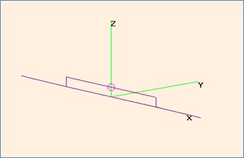
Figure 25 Tee Match NEC2 Model
The model parameters were set up as per step 1 ie. F = 299.8MHz, Free space, Dipole L/2 = 0.236m, rad = 0.001m. The Arm spacing is fixed at 25mm and arm diameter is the same as the Dipole. There was a variable defined for the arm length so that the model could be rerun several times with different arm lengths. Note the arm length in the table below is the length of one side or half the overall Tee length to facilitate comparisons with the Gamma case.
The following results were obtained:
|
Arm Wavelengths |
|
|
Zin T (Nec2) |
|
|
0.01 |
7+74.7j |
|
0.02 |
32.6+137j |
|
0.03 |
82.6+201j |
|
0.04 |
166+262j |
|
0.05 |
290+303j |
|
0.06 |
450+291j |
|
0.07 |
600+194j |
|
0.08 |
675+33.5j |
|
0.09 |
656-118j |
|
0.1 |
584-214j |
|
0.11 |
502-257j |
|
0.12 |
432-265j |
|
0.13 |
378-252j |
|
0.14 |
336-230j |
|
0.15 |
306-203j |
|
0.16 |
285-173j |
|
0.17 |
270-142j |
|
0.18 |
260-111j |
|
0.19 |
255-79.6j |
|
0.2 |
254-47.4j |
Table 2- TEE results from NEC2
Step 4. Compare NEC2 results to the Lumped/TL Model predictions.
The results are simplest compared in graphical form. The Gamma case is shown in Figure 26 and the Tee case in Figure 27.
Figure 26 Graph of Gamma NEC2 results vs TL model predictions.
Figure 27 Graph of Tee Nec2 results vs TL Model